The SQL Server "Segment Apply" Optimizer Transformations

Introduction

Almost 15 years ago (!), I wrote a short series of posts about Segment Apply (also known as Group By Apply):

• The “Segment Top” Query Optimization
• The Segment and Sequence Project Iterators
• Partitioning and the Common Subexpression Spool
• Ranking Function Optimizer Transformations

You’ll be familiar with the APPLY operator, which essentially represents logically repeating some action for each row of a source set. On each logical iteration, values from the current source row are made available to the inner side action as correlated parameters.

I stress that this is a logical operation because although this often results in a physical correlated nested loops implementation, that’s not always the case. The optimizer can often unnest a logical apply into a join, for example.

This article describes a more dramatic transformation of a logical apply.

Segment Apply

The idea of a Segment Apply is very similar to a regular APPLY, but instead of applying a repeating action for each row, we apply that action to a contiguous subset (a segment or group) of input rows.

For example, with Segment Top the idea is to take the first row (the repeated action) from each group (segment) of rows. We specify the logical grouping using T-SQL, a Segment physical plan operator identifies the start of each new group, and a Top operator returns one row from each identified group.

Example

Repeating the AdventureWorks example from my Segment Top article:

SELECT
    INV1.ProductID,
    INV1.LocationID,
    INV1.Shelf,
    INV1.Bin,
    INV1.Quantity
FROM Production.ProductInventory AS INV1
WHERE
    INV1.Quantity = 
    (
        -- Correlated to the outer
        -- query on Shelf and Bin
        SELECT
            min_qty = MIN(INV2.Quantity)
        FROM Production.ProductInventory AS INV2
        WHERE
            INV2.Shelf = INV1.Shelf
            AND INV2.Bin = INV1.Bin
    )
ORDER BY
    INV1.Shelf,
    INV1.Bin,
    INV1.Quantity;

Logic and implementation

This query logically says: Return details about the product with the lowest quantity in each bin on each shelf in the AdventureWorks product warehouse.

One way to physically implement that specification is to group the input rows by shelf and bin (forming a segment), then take the first row by quantity (the action) from each segment.

There are a couple of subtleties here:

1. We need to order the rows by shelf, bin, and quantity to ensure (shelf, bin) segments are contiguous and the lowest quantity appears first in each segment.

2. The TOP needs to be WITH TIES because there might be multiple products with the same minimum quantity in a particular bin. The original query would return all those tied matches, so the Segment Apply implementation must do that too.

The execution plan shows the main elements (sorting, segmenting, and the top):

We could avoid the sort with a suitable index of course. I didn’t do that here to show the sorting requirement more explicitly.

GenGbApplySimple

The Segment Top plan shape is just one of the alternatives that can be produced via the Segment Apply logic.

The GenGbApplySimple optimizer exploration rule recognises the logical idea of identifying segments in the data and repeating an action on them. One possible action is TOP (1) WITH TIES. The physical plan shape is ultimately constructed by the optimizer’s BuildGbApply implementation rule.

To see a different (non-top) action, let’s look again at another example from the Ranking Function Optimizer Transformations article:

SELECT
    INV.Bin,
    INV.Quantity,
    INV.ProductID,
    INV.Quantity,
    SubAgg.total_in_bin
FROM Production.ProductInventory AS INV
JOIN
(
    -- Calculates the total quantity in each bin
    SELECT
        INV2.Shelf,
        INV2.Bin,
        total_in_bin = SUM(INV2.Quantity)
    FROM Production.ProductInventory AS INV2
    GROUP BY
        INV2.Shelf,
        INV2.Bin
) AS SubAgg
    ON SubAgg.Shelf = INV.Shelf
    AND SubAgg.Bin = INV.Bin
WHERE
    INV.Shelf >= N'A' 
    AND INV.Shelf <= N'C'
ORDER BY
    INV.Shelf,
    INV.Bin;

This time, we’re looking for product details plus the total quantity of all products in the same bin. The SQL representation is quite verbose but it boils down to splitting the rows into (shelf, bin) segments and repeating a SUM(Quantity) action for each segment.

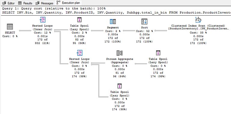
This logical equivalence is recognised by the GenGbApplySimple rule. Again, sorting is necessary and could be provided by an index. The execution plan (built in part by BuildGbApply) is quite different from the Segment Top seen before:

Now we have a Segment Spool plan.

• The Sort ensures rows are in (shelf, bin) order suitable for segmenting.
• The Segment operator identifies the start of a new segment.
• The Spool after the Segment saves the current segment of rows.
• The other spools are secondary spools, replaying the current segment to compute the required aggregate, then adding that aggregate as a new column for each row in the current segment via a cross join.

This is the most literal representation of Segment Apply. A segment of rows is stored in a spool and then replayed for each applied action. If you want all the fine details about how this plan executes, please see the prior articles.

Although this plan looks very different from the Segment Top, it is logically very similar and produced by the same optimizer exploration rules.

GenGbApplyAgg

There is another exploration rule that can recognise the Segment Apply pattern, but I didn’t have a simple reproduction query for it until just recently.

As the name suggests, GenGbApplyAgg recognises a similar pattern but with the presence of an additional layer of aggregation. The logical transform is:

Join(GbAgg(x), GbAgg(GbAgg(x))) -> GbApply(GbAgg(x))

That’s probably not intuitively clear for most people, so let’s look at an example.

Segment aggregate apply example

Say we need to identify bins in the AdventureWorks warehouse that contain less than 25% of the average number of parts for all bins on the same shelf.

That’s quite a complex requirement, so we might start by breaking it down into simpler steps and aggregations.

First, the total quantity of parts per bin and shelf:

-- Total quantity per bin & shelf (TQBS)
SELECT
    INV.Shelf,
    INV.Bin,
    BinTotal = SUM(INV.Quantity)
FROM Production.ProductInventory AS INV
GROUP BY
    INV.Shelf,
    INV.Bin

Next, the average bin total per shelf, reusing the prior result:

-- Average bin total per shelf (APS)
SELECT
    TQBS.Shelf,
    BinAvg = AVG(TQBS.BinTotal)
FROM TQBS
GROUP BY
    TQBS.Shelf

With those two intermediate results expressed as Common Table Expressions (CTEs), we can now write the final query:

SELECT
    TQBS.Shelf, 
    TQBS.Bin, 
    TQBS.BinTotal,
    APS.BinAvg,
    Pct = TQBS.BinTotal * 100.0 / APS.BinAvg
FROM TQBS
JOIN APS
    -- Same shelf
    ON APS.Shelf = TQBS.Shelf
WHERE
    -- Bin has less than 25% of the shelf average
    TQBS.BinTotal < APS.BinAvg * 0.25

The finished query

Putting it all together in one big executable query:

WITH
    TQBS AS
    (
        -- Total quantity per bin & shelf
        SELECT
            INV.Shelf,
            INV.Bin,
            BinTotal = SUM(INV.Quantity)
        FROM Production.ProductInventory AS INV
        GROUP BY
            INV.Shelf,
            INV.Bin
    ),
    APS AS
    (
        -- Average bin total per shelf
        -- References the previous CTE
        SELECT
            TQBS.Shelf,
            BinAvg = AVG(TQBS.BinTotal)
        FROM TQBS
        GROUP BY
            TQBS.Shelf
    )
SELECT
    TQBS.Shelf, 
    TQBS.Bin, 
    TQBS.BinTotal,
    APS.BinAvg,
    Pct = TQBS.BinTotal * 100.0 / APS.BinAvg
FROM TQBS
JOIN APS
    -- Same shelf
    ON APS.Shelf = TQBS.Shelf
WHERE
    -- Bin has less than 25% of the shelf average
    TQBS.BinTotal < APS.BinAvg * 0.25
ORDER BY
    TQBS.Shelf, 
    TQBS.Bin;

That’s a moderately complex query with a join between one CTE and another, where one CTE also operates on the results of the other. There are multiple CTE references, so we might expect multiple base table accesses as a result, and quite a complicated plan overall.

Execution plan

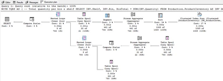
The plan is surprisingly simple (and familiar):

The main difference from the shape we saw earlier is that this plan has an aggregate between the Sort and the Segment. Hence the Agg in the GenGbApplyAgg name instead of Simple.

Notice in particular that the base table is only accessed once despite the join and multiple CTE references.

A brief outline of how this plan works:

• The Sort puts the rows into (Shelf, Bin) order for aggregation and segmenting.
• The Stream Aggregate after the Sort computes SUM(Quantity) per shelf and bin.
• The Segment identifies the start of a new segment.
• The top Spool holds the current segment of rows.
• The Stream Aggregate after the middle spool replay computes the SUM and COUNT using the previously computed SUM(Quantity) for all rows in the current segment.
• The following Compute Scalar computes AVG using the new SUM and COUNT.
• The final Spool replays segment rows to cross join the scalar AVG result onto them.
• The final top-level Compute Scalar calculates the percentage.

Window function

If you’re the sort of person that enjoys complex window aggregates, you might recognise the average computation above as being equivalent to the following T-SQL syntax:

SELECT
    Q1.Shelf, 
    Q1.Bin, 
    Q1.BinTotal, 
    Q1.BinAvg,
    Pct = Q1.BinTotal * 100.0 / Q1.BinAvg
FROM 
(
    SELECT
        INV.Shelf,
        INV.Bin,
        BinTotal = 
            SUM(INV.Quantity),
        BinAvg = 
            -- Yikes!
            AVG(SUM(INV.Quantity)) OVER (
            PARTITION BY INV.Shelf)
    FROM Production.ProductInventory AS INV
    GROUP BY 
        INV.Shelf, 
        INV.Bin
) AS Q1
WHERE
    Q1.BinTotal < Q1.BinAvg * 0.25
ORDER BY
    Q1.Shelf,
    Q1.Bin;

That way of writing the query produces the same results as with multiple CTEs. The execution plan is also logically equivalent, despite the very different T-SQL syntax:

The only difference is the separate Filter for the 25% comparison. The multiple CTE query form successfully pushed this predicate down to the middle cross join of the common subexpression spool subtree, which is a tiny bit more efficient than the windowing query’s plan.

Regardless of your preference for multiple CTEs over a window function on an aggregate, it’s pretty remarkable that the optimizer can recognise the logic here and apply (ha) the same Segment Apply transformation in both cases.

Closing Remarks

The examples above work on every edition of AdventureWorks from SQL Server 2008 R2 onward. As my 15-year-old articles testify, the Segment Apply optimization has been available for a very long time.

It can sometimes be difficult to write a query that matches the Segment Apply pattern and there’s no feedback when SQL Server refuses. Note also that a Segment Apply is just one alternative and the optimizer might choose something else for estimated cost reasons.

It’s a bit of a shame that this capability hasn’t been expanded over time. There’s no batch mode Window Aggregate implementation, for example.

The spool-based row mode implementation often provides adequate performance and the single table access can be a significant benefit.

There are no batch mode spools and they don’t have bulk optimizations like temporary tables, so performance can be limited with higher row counts. Likewise, there’s no batch mode Segment or Top operator.

Still, I hope you found these details interesting.

Thanks for reading.