Join Cardinality Estimation using Histogram Coarse Alignment

Introduction

The primary changes made to Cardinality Estimation starting with the SQL Server 2014 release are described in the Microsoft White Paper Optimizing Your Query Plans with the SQL Server 2014 Cardinality Estimator by Joe Sack, Yi Fang, and Vassilis Papadimos.

One of those changes concerns the estimation of simple joins with a single equality or inequality predicate using statistics histograms. In the section headed, “Join Estimate Algorithm Changes”, the paper introduced the concept of “coarse alignment” using minimum and maximum histogram boundaries:

For joins with a single equality or inequality predicate, the legacy CE joins the histograms on the join columns by aligning the two histograms step-by-step using linear interpolation. This method could result in inconsistent cardinality estimates. Therefore, the new CE now uses a simpler join estimate algorithm that aligns histograms using only minimum and maximum histogram boundaries.

Although potentially less consistent, the legacy CE may produce slightly better simple-join condition estimates because of the step-by-step histogram alignment. The new CE uses a coarse alignment. However, the difference in estimates may be small enough that it will be less likely to cause a plan quality issue.

As one of the technical reviewers of the paper, I felt that a little more detail around this change would have been useful, but that did not make it into the final version. This article adds some of that detail.

Coarse Histogram Alignment Example

The coarse alignment example in the White Paper uses the Data Warehouse version of the AdventureWorks sample database. Despite the name, the database is rather small; the backup is only 22.3MB and expands to around 200MB. It can be downloaded via links on the AdventureWorks Installation and Configuration documentation page.

The query we are interested in joins the FactResellerSales and FactCurrencyRate tables.

SELECT
    FRS.ProductKey,
    FRS.OrderDateKey,
    FRS.DueDateKey,
    FRS.ShipDateKey,
    FCR.DateKey,
    FCR.AverageRate,
    FCR.EndOfDayRate,
    FCR.[Date]
FROM dbo.FactResellerSales AS FRS
JOIN dbo.FactCurrencyRate AS FCR
    ON FCR.CurrencyKey = FRS.CurrencyKey;

This is a simple equijoin on a single column so it qualifies for join cardinality and selectivity estimation using histogram coarse alignment.

Histograms

The histograms we need are associated with the CurrencyKey column on each joined table. On a fresh copy of the AdventureWorksDW database, the pre-existing statistics for the larger FactResellerSales table are based on a sample. To maximize reproducibility and make the detailed calculations as simple as possible to follow (avoiding scaling), the first thing we will do is to refresh the statistics using a full scan:

UPDATE STATISTICS dbo.FactCurrencyRate WITH FULLSCAN;
UPDATE STATISTICS dbo.FactResellerSales WITH FULLSCAN;

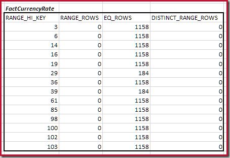
These tables have the demo-friendly benefit of creating small and simple maxdiff histograms:

DBCC SHOW_STATISTICS
    (FactResellerSales, CurrencyKey)
WITH HISTOGRAM;

DBCC SHOW_STATISTICS
    (FactCurrencyRate, [PK_FactCurrencyRate_CurrencyKey_DateKey])
WITH HISTOGRAM;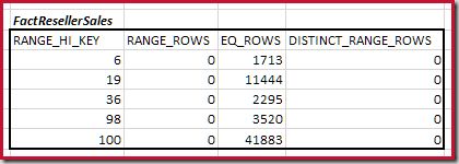

Combining Minimum Matching Histogram Steps

The first step in the coarse alignment calculation is to find the contribution to the join cardinality provided by the lowest matching histogram step. For our example histograms, the minimum matching step value is on RANGE_HI_KEY = 6:

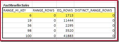
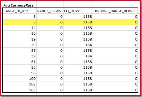
The estimated equijoin cardinality for just this highlighted step is 1,713 * 1,158 = 1,983,654 rows.

Remaining Matched Steps

Next, we need to identify the range of histogram RANGE_HI_KEY steps up to the maximum for possible equijoin matches. This involves moving forward from the previously-found minimum until one of the histogram inputs runs out of rows. The matching equijoin ranges for the current example are highlighted below:

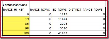
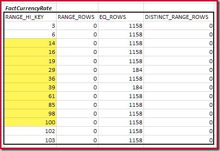
These two ranges represent the remaining rows that may be expected to contribute to equijoin cardinality.

Coarse Frequency-Based Estimation

The question is now how to perform a coarse estimation of the equijoin cardinality of the highlighted steps, using the information available.

The original cardinality estimator would have performed a fine-grained step-by-step histogram alignment using linear interpolation, assessed the join contribution of each step (much as we did for the minimum step value before), and summed each step contribution to acquire a full join estimate. While this procedure makes a lot of intuitive sense, practical experience was that this fine-grained approach added computational overhead and could produce results of variable quality.

The original estimator had another way to estimate join cardinality when histogram information was either not available, or heuristically assessed to be inferior. This is known as a frequency-based estimation, and uses the following definitions:

• C – the cardinality (number of rows)
• D – the number of distinct values
• F – the frequency (number of rows) for each distinct value
• Note C = D * F by definition

The effect of an equijoin of relations R1 and R2 on each of these properties is as shown below:

• F’ = F1 * F2
• D’ = MIN(D1; D2) – assuming containment
• C’ = D’ * F’ (again, by definition)

We are after C’, the cardinality of the equijoin. Substituting for D’ and F’ in the formula, and expanding:

• C’ = D’ * F’
• C’ = MIN(D1; D2) * F1 * F2
• C’ = MIN(D1 * F1 * F2; D2 * F1 * F2)
• now, since C1 = D1 * F1, and C2 = D2 * F2:
• C’ = MIN(C1 * F2, C2 * F1)
• finally, since F = C/D (also by definition):
• C’ = MIN(C1 * C2 / D2; C2 * C1 / D1)

Noting that C1 * C2 is the product of the two input cardinalities (Cartesian join), it is clear that the minimum of those expressions will be the one with the higher number of distinct values:

• C’ = (C1 * C2) / MAX(D1; D2)

In case this all seems a little abstract, an intuitive way to think about frequency-based equijoin estimation is to consider that each distinct value from one relation will join with a number of rows (the average frequency) in the other relation. If we have 5 distinct values on one side, and each distinct value on the other side appears 3 times on average, a sensible (but coarse) equijoin estimate is 5 * 3 = 15.

This is not quite such a broad brush as it might appear. Remember the cardinality and distinct values numbers above come not from the whole relation, but only from the matching steps above the minimum. Hence coarse estimation between minimum and maximum values.

Frequency Calculation

We can get each of these parameters from the highlighted histogram steps.

• The cardinality C is the sum of EQ_ROWS and RANGE_ROWS.
• The number of distinct values D is the sum of DISTINCT_RANGE_ROWS plus one for each step.

The cardinality C1 of matching FactResellerSales steps is the sum of the cells highlighted:

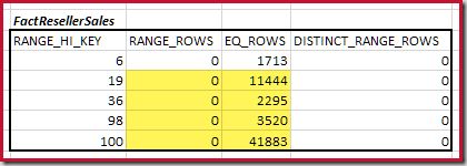
This gives C1 = 59,142 rows.

There are no distinct range rows, so the only distinct values come from the four step boundaries themselves, giving D1 = 4.

For the second table:

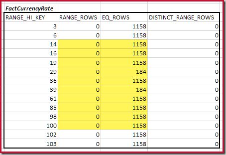
This gives C2 = 9,632. Again there are no distinct range rows, so the distinct values come from the ten step boundaries, D2 = 10.

Completing the Equijoin Estimate

We now have all the numbers we need for the equijoin formula:

• C’ = (C1 * C2) / MAX(D1; D2)
• C’ = (59142 * 9632) / MAX(4; 10)
• C’ = 569655744 / 10
• C’ = 56,965,574.4

Remember, this is the contribution of the histogram steps above the minimum matched boundary. To complete the join cardinality estimation we need to add in the contribution from the minimum matching step values, which was 1,713 * 1,158 = 1,983,654 rows.

The final equijoin estimate is therefore 56,965,574.4 + 1,983,654 = 58,949,228.4 rows or 58,949,200 to six significant figures.

This result is confirmed in the estimated execution plan for the source query:

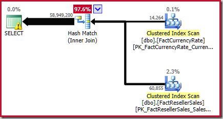
As noted in the White Paper, this is not a great estimate. The actual number of rows returned by this query is 70,470,090. The estimate produced by the original (“legacy”) cardinality estimator – using step-by-step histogram alignment – is 70,470,100 rows.

Better results are often possible with the finer method, but only if the statistics are a very good representation of the underlying data distribution. This is not simply a matter of keeping statistics up to date, or using full scan population. The algorithm used to pack information into a maximum of 201 histogram steps is not perfect, and in any case many real-world data distributions simply aren’t capable of such histogram fidelity. On average, people should find that the coarser method provides perfectly adequate estimations and greater stability with the new CE.

Second Example

This builds a little on the previous example, and does not require a sample database download.

DROP TABLE IF EXISTS
    dbo.R1,
    dbo.R2;

CREATE TABLE dbo.R1 (n integer NOT NULL);
CREATE TABLE dbo.R2 (n integer NOT NULL);

INSERT dbo.R1
    (n)
VALUES
    (1), (2), (3), (4), (5), (6), (7), (8), (9), (10),
    (6), (6), (6), (6), (6), (6), (6), (6), (6), (6), 
    (6), (6), (6), (6), (6), (6), (6), (6), (6);

INSERT dbo.R2
    (n)
VALUES
    (5), (6), (7), (8), (9), (10), (11), (12), (13), (14), (15),
    (10), (10);

CREATE STATISTICS stats_n ON dbo.R1 (n) WITH FULLSCAN;
CREATE STATISTICS stats_n ON dbo.R2 (n) WITH FULLSCAN;

The histograms showing matched minimum steps are:

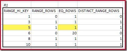
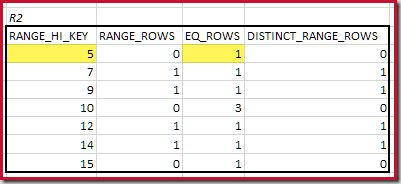
The lowest RANGE_HI_KEY that matches is 5. The value of EQ_ROWS is 1 in both, so the estimated equijoin cardinality is 1 * 1 = 1 row.

The highest matching RANGE_HI_KEY is 10. Highlighting the R1 histogram rows for coarse frequency-based estimation:

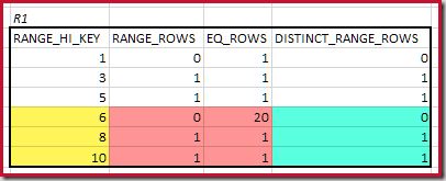
Summing EQ_ROWS and RANGE_ROWS gives C1 = 24. The number of distinct rows is 2 DISTINCT_RANGE_ROWS (distinct values between steps) plus 3 for the distinct values associated with each step boundary, giving D1 = 5.

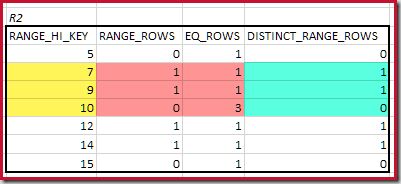
For R2, summing EQ_ROWS and RANGE_ROWS gives C2 = 7. The number of distinct rows is 2 DISTINCT_RANGE_ROWS (distinct values between steps) plus 3 for the distinct values associated with each step boundary, giving D2 = 5.

The equijoin estimate C’ is:

• C’ = (C1 * C2) / MAX(D1; D2)
• C’ = (24 * 7) / 5
• C’ = 33.6

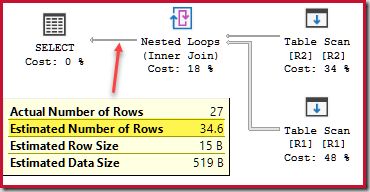
Adding in the 1 row from the minimum step match gives a total estimate of 34.6 rows for the equijoin:

SELECT
    R1.n,
    R2.n
FROM dbo.R1 AS R1
JOIN dbo.R2 AS R2
    ON R2.n = R1.n;

The estimated execution plan shows an estimate matching our calculation:

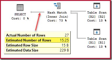
This is not exactly right, but the “legacy” cardinality estimator does no better, estimating 15.25 rows versus 27 actual:

For a complete treatment, we would also have to add in a final contribution from matching histogram null steps, but this is uncommon for equijoins (which are typically written to reject nulls) and a relatively straightforward extension for the interested reader.

Final Thoughts

Hopefully the details in the article will fill in a few gaps for anyone who has ever wondered about “coarse alignment.” Note that this is just one small component in the cardinality estimator. There are several other important concepts and algorithms used for join estimation, notably the way that non-join predicates are assessed, and how more complex joins are handled. Many of the really important bits are pretty well covered in the White Paper.

Thanks for reading.