Performance Tuning the Whole Query Plan

Introduction

Execution plans provide a rich source of information that can help us identify ways to improve the performance of important queries. People often look for things like large scans and lookups as a way to identify potential data access path optimizations. These issues can often be quickly resolved by creating a new index or extending an existing one with more included columns.

We can also use post-execution plans to compare actual with expected row counts between plan operators. Where these are found to be significantly at variance, we can try to provide better statistical information to the optimizer by updating existing statistics, creating new statistics objects, utilizing statistics on computed columns, or perhaps by breaking a complex query up into less-complex component parts.

Beyond that, we can also look at expensive operations in the plan, particularly memory-consuming ones like sorting and hashing. Sorting can sometimes be avoided through indexing changes. Other times, we might have to refactor the query using syntax that favours a plan that preserves a particular desired ordering.

Sometimes, performance will still not be good enough even after all these performance tuning techniques are applied. A possible next step is to think a bit more about the plan as a whole. This means taking a step back, trying to understand the overall strategy chosen by the query optimizer, to see if we can identify an algorithmic improvement.

This article explores this latter type of analysis, using a simple example problem of finding unique column values in a moderately large data set. As is often the case in analogous real-world problems, the column of interest will have relatively few unique values, compared with the number of rows in the table. There are two parts to this analysis: creating the sample data, and writing the distinct-values query itself.

Creating the Sample Data

To provide the simplest possible example, our test table has just a single column with a clustered index (this column will hold duplicate values so the index cannot be declared unique):

CREATE TABLE dbo.Test 
(
    data integer NOT NULL,
);
GO
CREATE CLUSTERED INDEX cx
ON dbo.Test (data);

To pick some numbers out of the air, we will choose to load ten million rows in total, with an even distribution over a thousand distinct values. A common technique to generate data like this is to cross join some system tables and apply the ROW_NUMBER function. We will also use the modulo operator to limit the generated numbers to the desired distinct values:

INSERT dbo.Test WITH (TABLOCK)
    (data)
SELECT TOP (10000000)
    (ROW_NUMBER() OVER (ORDER BY (SELECT 0)) % 1000) + 1
FROM master.sys.columns AS C1 WITH (READUNCOMMITTED)
CROSS JOIN master.sys.columns AS C2 WITH (READUNCOMMITTED)
CROSS JOIN master.sys.columns C3 WITH (READUNCOMMITTED);

The estimated execution plan for that query is as follows (click the image to enlarge it if necessary):

This takes around 30 seconds to create the sample data on my laptop. That is not an enormous length of time by any means, but it is still interesting to consider what we might do to make this process more efficient…

Plan analysis

We will start by understanding what each operation in the plan is there for.

The section of the execution plan to the right of the Segment operator is concerned with manufacturing rows by cross joining system tables:

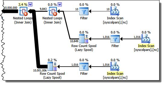
The Segment operator is there in case the window function had a PARTITION BY clause. That is not the case here, but it features in the query plan anyway. The Sequence Project operator generates the row numbers, and the Top limits the plan output to ten million rows:

The Compute Scalar defines the expression that applies the modulo function and adds one to the result:

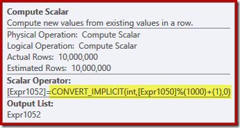
We can see how the Sequence Project and Compute Scalar expression labels relate using Plan Explorer’s Expressions tab:

This gives us a more complete feel for the flow of this plan: the Sequence Project numbers the rows and labels the expression Expr1050; the Compute Scalar labels the result of the modulo and plus-one computation as Expr1052. Notice also the implicit conversion in the Compute Scalar expression. The destination table column is of type integer, whereas the ROW_NUMBER function produces a bigint, so a narrowing conversion is necessary.

The next operator in the plan is a Sort. According to the query optimizer’s costing estimates, this is expected to be the most expensive operation (88.1% estimated):

It might not be immediately obvious why this plan features sorting, since there is no explicit ordering requirement in the query. The Sort is added to the plan to ensure rows arrive at the Clustered Index Insert operator in clustered index order. This promotes sequential writes, avoids page splitting, and is one of the pre-requisites for minimally-logged INSERT operations.

These are all potentially good things, but the Sort itself is rather expensive. Indeed, checking the post-execution (“actual”) execution plan reveals the Sort also ran out of memory at execution time and had to spill to physical tempdb disk:

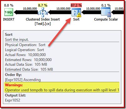
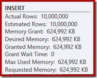
The Sort spill occurs despite the estimated number of rows being exactly right, and despite the fact the query was granted all the memory it asked for (as seen in the plan properties for the root INSERT node):

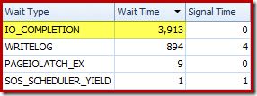
Sort spills are also indicated by the presence of IO_COMPLETION waits in the Plan Explorer wait stats tab:

Finally for this plan analysis section, notice the DML Request Sort property of the Clustered Index Insert operator is set true:

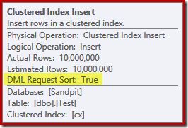
This flag indicates that the optimizer requires the sub-tree below the Insert to provide rows in index key sorted order (hence the need for the problematic Sort operator).

Avoiding the sort

Now that we know why the Sort appears, we can test to see what happens if we remove it. There are ways we could rewrite the query to “fool” the optimizer into thinking fewer rows would be inserted (so sorting would not be worthwhile) but a quick way to avoid the sort directly (for experimental purposes only) is to use undocumented trace flag 8795. This sets the DML Request Sort property to false, so rows are no longer required to arrive at the Clustered Index Insert in clustered key order:

TRUNCATE TABLE dbo.Test;
GO
INSERT dbo.Test WITH (TABLOCK)
    (data)
SELECT TOP (10000000)
    ROW_NUMBER() OVER (ORDER BY (SELECT 0)) % 1000
FROM master.sys.columns AS C1 WITH (READUNCOMMITTED)
CROSS JOIN master.sys.columns AS C2 WITH (READUNCOMMITTED)
CROSS JOIN master.sys.columns C3 WITH (READUNCOMMITTED)
OPTION (QUERYTRACEON 8795);

The new post-execution query plan is as follows (click the image to enlarge):

The Sort operator has gone, but the new query runs for over 50 seconds (compared with 30 seconds before). There are a couple of reasons for this. First, we lose any possibility of minimally-logged inserts because these require sorted data (DML Request Sort = true). Second, a large number of “bad” page splits will occur during the insert. In case that seems counter-intuitive, remember that although the ROW_NUMBER function numbers rows sequentially, the effect of the modulo operator is to present a repeating sequence of numbers 1…1000 to the Clustered Index Insert.

The same fundamental issue occurs if we use T-SQL tricks to lower the expected row count to avoid the sort instead of using the unsupported trace flag.

Avoiding the sort II

Looking at the plan as a whole, it seems clear we would like to generate rows in a way that avoids an explicit sort, but which still reaps the benefits of minimal logging and bad page split avoidance. Put simply: we want a plan that presents rows in clustered key order, but without sorting.

Armed with this new insight, we can express our query in a different way. The following query generates each number from 1 to 1000 and cross joins that set with 10,000 rows to produce the required degree of duplication. The idea is to generate an insert set that presents 10,000 rows numbered ‘1’ then 10,000 numbered ‘2’ … and so on.

TRUNCATE TABLE dbo.Test;
GO
INSERT dbo.Test WITH (TABLOCK)
    (data)
SELECT 
    N.number 
FROM 
(
    SELECT SV.number
    FROM master.dbo.spt_values AS SV WITH (READUNCOMMITTED)
    WHERE SV.[type] = N'P'
    AND SV.number >= 1
    AND SV.number <= 1000
) AS N
CROSS JOIN
(
    SELECT TOP (10000)
        Dummy = NULL
    FROM master.sys.columns AS C1 WITH (READUNCOMMITTED)
    CROSS JOIN master.sys.columns AS C2 WITH (READUNCOMMITTED)
    CROSS JOIN master.sys.columns C3 WITH (READUNCOMMITTED)
) AS C;

Unfortunately, the optimizer still produces a plan with a sort:

There is not much to be said in the optimizer’s defense here, this is just a daft plan. It has chosen to generate 10,000 rows then cross join those with numbers from 1 to 1000. This does not allow the natural order of the numbers to be preserved, so the sort cannot be avoided.

Avoiding the sort, finally

The strategy the optimizer missed is to take the numbers 1…1000 first, and cross join each number with 10,000 rows (making 10,000 copies of each number in sequence). The expected plan would avoid a sort by using a nested loops cross join that preserves the order of the rows on the outer input.

We can achieve this outcome by forcing the optimizer to access the derived tables in the order specified in the query, using the FORCE ORDER query hint:

TRUNCATE TABLE dbo.Test;
GO
INSERT dbo.Test WITH (TABLOCK)
    (data)
SELECT 
    N.number 
FROM 
(
    SELECT SV.number
    FROM master.dbo.spt_values AS SV WITH (READUNCOMMITTED)
    WHERE SV.[type] = N'P'
    AND SV.number >= 1
    AND SV.number <= 1000
) AS N
CROSS JOIN
(
    SELECT TOP (10000)
        Dummy = NULL
    FROM master.sys.columns AS C1 WITH (READUNCOMMITTED)
    CROSS JOIN master.sys.columns AS C2 WITH (READUNCOMMITTED)
    CROSS JOIN master.sys.columns C3 WITH (READUNCOMMITTED)
) AS C
OPTION (FORCE ORDER);

Finally, we get the plan we were after:

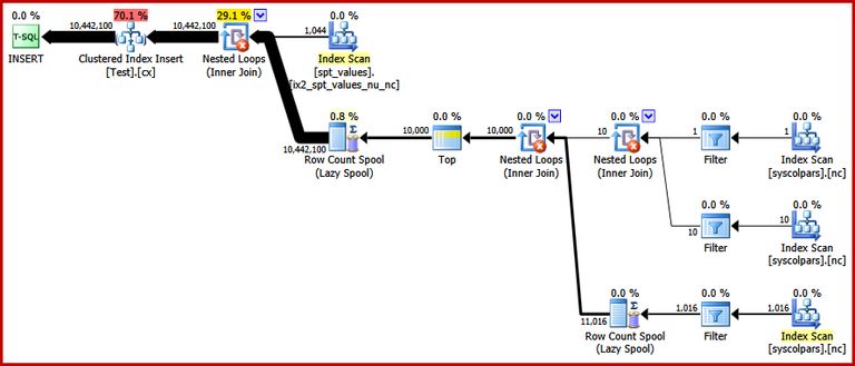
This plan avoids an explicit sort while still avoiding “bad” page splits and enabling minimally-logged inserts to the clustered index (assuming the database is not using the FULL recovery model). It loads all ten million rows in about 9 seconds on my laptop (with a single 7200 rpm SATA spinning disk). This represents a marked efficiency gain over the 30-50 second elapsed time seen before the rewrite.

Finding Distinct Values

Now we have the sample data created, we can turn our attention to writing a query to find the distinct values in the table. A natural way to express this requirement in T-SQL is as follows:

SELECT DISTINCT data
FROM dbo.Test WITH (TABLOCK)
OPTION (MAXDOP 1);

The execution plan is very simple, as you would expect:

This takes around 2900 ms to run on my machine, and requires 43,406 logical reads:

Removing the MAXDOP (1) query hint generates a parallel plan:

This completes in about 1500 ms (but with 8,764 ms of CPU time consumed), and 43,804 logical reads:

The same plans and performance result if we use GROUP BY instead of DISTINCT.

A Better Algorithm

The query plans shown above read all values from the base table and process them through a Stream Aggregate. Thinking of the task as a whole, it seems inefficient to scan all 10 million rows when we know there are relatively few distinct values.

A better strategy might be to find the single lowest value in the table, then find the next highest, and so on until we run out of values. Crucially, this approach lends itself to singleton-seeking into the index rather than scanning every row.

We can implement this idea in a single query using a recursive CTE, where the anchor part finds the lowest distinct value, then the recursive part finds the next distinct value and so on. A first attempt at writing this query is:

WITH RecursiveCTE
AS
(
    -- Anchor
    SELECT data = MIN(T.data)
    FROM dbo.Test AS T

    UNION ALL

    -- Recursive
    SELECT MIN(T.data)
    FROM dbo.Test AS T
    JOIN RecursiveCTE AS R
        ON R.data < T.data
)
SELECT data
FROM RecursiveCTE
OPTION (MAXRECURSION 0);

Unfortunately, that syntax does not compile:

Ok, so aggregate functions are not allowed. Instead of using MIN, we can write the same logic using TOP (1) with an ORDER BY:

WITH RecursiveCTE
AS
(
    -- Anchor
    SELECT TOP (1)
        T.data
    FROM dbo.Test AS T
    ORDER BY
        T.data

    UNION ALL

    -- Recursive
    SELECT TOP (1)
        T.data
    FROM dbo.Test AS T
    JOIN RecursiveCTE AS R
        ON R.data < T.data
    ORDER BY T.data
)
SELECT 
    data
FROM RecursiveCTE
OPTION (MAXRECURSION 0);

Still no joy.

It turns out that we can get around these restrictions by rewriting the recursive part to number the candidate rows in the required order, then filter for the row that is numbered ‘one’. This might seem a little circuitous, but the logic is exactly the same:

WITH RecursiveCTE
AS
(
    -- Anchor
    SELECT TOP (1)
        data
    FROM dbo.Test AS T
    ORDER BY
        T.data

    UNION ALL

    -- Recursive
    SELECT R.data
    FROM
    (
        -- Number the rows
        SELECT 
            T.data,
            rn = ROW_NUMBER() OVER (
                ORDER BY T.data)
        FROM dbo.Test AS T
        JOIN RecursiveCTE AS R
            ON R.data < T.data
    ) AS R
    WHERE
        -- Only the row that sorts lowest
        R.rn = 1
)
SELECT 
    data
FROM RecursiveCTE
OPTION (MAXRECURSION 0);

This query does compile, and produces the following post-execution plan:

Notice the Top operator in the recursive part of the execution plan (highlighted). We cannot write a T-SQL TOP in the recursive part of a recursive common table expression, but that does not mean the optimizer cannot use one! The optimizer introduces the Top based on reasoning about the number of rows it will need to check to find the one numbered ‘1’.

The performance of this (non-parallel) plan is much better than the Stream Aggregate approach. It completes in around 50 ms, with 3007 logical reads against the source table (and 6001 rows read from the spool worktable), compared with the previous best of 1500ms (8764 ms CPU time at DOP 8) and 43,804 logical reads:

Conclusion

It is not always possible to achieve breakthroughs in query performance by considering individual query plan elements on their own. Sometimes, we need to analyse the strategy behind the whole execution plan, then think laterally to find a more efficient algorithm and implementation.

Thanks for reading.