Query Optimizer Deep Dive—Part 2

This is the second in a series of posts based on the content of the Query Optimizer Deep Dive presentations I have given over the last month or so at the Auckland SQL Users’ Group, and SQL Saturday events in Wellington, New Zealand and Adelaide, Australia.

Cost-Based Optimization Overview

The input to cost-based optimization is a tree of logical operations produced by the previous optimization stages discussed in part one.

Cost-based optimization takes this logical tree, explores logical alternatives (different logical tree shapes that will always produce the same results), generates physical implementations, assigns an estimated cost to each, and finally chooses the cheapest physical option overall.

The goal of cost-based optimization is not to find the best possible physical execution plan by exploring every possible alternative. Rather, the goal is to find a good plan quickly.

This approach gives us an optimizer that works pretty well for most workloads, most of the time. If you think about it, that’s quite an achievement — after all, my database is likely very different from yours, and we probably run on quite different hardware as well. The point about finding a good plan quickly is also important. Generally, we would not want the optimizer to spend hours optimizing a query that runs for only a few seconds.

This design has a number of important consequences. First, a skilled query tuner will often be able to come up with a better plan than the optimizer does. In some cases, this will because the human can reason about the query in a way the optimizer cannot. Other times, it is simply a question of time — we might be happy spending half a day finding a great execution plan for a crucial query, whereas the optimizer places strict limits on itself to avoid spending more time on optimization than it saves on a single execution.

Perhaps a future version of SQL Server will allow us to configure the optimizer to spend extra time on a particular query. Today, we have to use query hints and ‘manual optimizations’ to encourage a particular execution plan shape.

The down side to circumventing the optimizer’s natural behaviour in this way is that we then have to take responsibility for ensuring that the execution plan remains good in the future, as data volumes and distributions change. In most systems, it is best to limit the number of manually-tuned queries to a minimum, and thoroughly document any tricks you use to obtain a particular plan.

Input Tree to Cost-Based Optimization

Back to the task at hand. We have an AdventureWorks query (reproduced below) that has been through all the previous optimization stages, did not qualify for a trivial plan, and so needs to go through the cost-based optimization process.

SELECT
    P.[Name],
    Total = SUM(INV.Quantity)
FROM 
    Production.Product AS P,
    Production.ProductInventory AS INV
WHERE
    INV.ProductID = P.ProductID
    AND P.[Name] LIKE N'[A-G]%'
GROUP BY
    P.[Name];

The tree of logical operations passed to the optimizer looks like this:

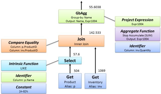
This looks very similar to the original logical tree seen in part one, though cardinality estimates have been added to each primary node, and the tree layout has been expanded a little into a form that is easier for the system to work with.

In addition to simple cardinality estimates, remember that each node also has statistics objects (histograms and frequency information) derived from the familiar statistics associated with the tables in the query.

The tree above was built from information obtained using trace flag 3604 and 8606 (see part one for more details). Trace flag 8606 shows the tree at various stages, the diagram above is built from the view after project normalization:

*** Tree After Project Normalization ***
LogOp_GbAgg OUT(QCOL: [P].Name,COL: Expr1002 ,) BY(QCOL: [P].Name,)
    LogOp_Join
        LogOp_Select
            LogOp_Get TBL: Production.Product(alias TBL: P)
            ScaOp_Intrinsic like
                ScaOp_Identifier QCOL: [P].Name
                ScaOp_Const TI(nvarchar collate 872468488,Var,Trim,ML=12)
                ScaOp_Const TI(nvarchar collate 872468488,Var,Trim,ML=2)
                ScaOp_Const TI(nvarchar collate 872468488,Null,Var,Trim,ML=12)
                ScaOp_Const TI(nvarchar collate 872468488,Null,Var,Trim,ML=12)
                ScaOp_Const TI(int,Null,ML=4) XVAR(int,Not Owned,Value=30)
        LogOp_Get TBL: Production.ProductInventory(alias TBL: INV) Production.ProductInventory
        ScaOp_Comp x_cmpEq
            ScaOp_Identifier QCOL: [P].ProductID
            ScaOp_Identifier QCOL: [INV].ProductID
    AncOp_PrjList 
        AncOp_PrjEl COL: Expr1002 
            ScaOp_AggFunc stopAccum
                ScaOp_Identifier QCOL: [INV].Quantity

Properties

There are a number of other ‘properties’ associated with each node, added by previous optimization work. These properties include logical attributes, such as:

• Output columns and expressions
• Uniqueness (key) information
• Type information and nullability
• Functional dependencies
• Domain ranges for each column or expression

There are also some physical properties that may be present on each node, for example:

• Sort order at each node
• Partitioning information
• Halloween protection

The Halloween protection information is worth explaining in a bit more detail. A row-mode query generally executes as a pipeline, with rows being requested one at a time from the top of the tree, so rows are in effect pulled up the tree one at a time.

This pipeline arrangement has a number of important advantages, but a problem can arise where the query modifies data. Changes made by the query can affect rows being read by the same query.

The classic example is a query that adds 10% to the salaries of every employee. When processed as a pipeline, we can get stuck in an infinite loop as rows that have had 10% added re-qualify for reading. This problem happened to be first discovered on 31 October 1976 and became known as the Halloween Problem.

One solution is to fully separate operations that read data from those that update data by reading all rows into temporary storage before performing any updates. In SQL Server, this simple solution typically manifests as an Eager Table Spool in the query plan. All rows are written eagerly to temporary storage before any updates are performed.

This is a bit of a sledgehammer solution though, so the optimizer keeps track of which columns need protection from the Halloween problem (and how much protection they need) at each node by setting properties. Some logical operations (like sorting) naturally mean that all input rows have to be read before the first output row can be produced.

These operations provide Halloween protection naturally, so an explicit Eager Table Spool would not be necessary. There are a number of logical operations that can provide some degree of Halloween protection, and properties are used to ensure that just enough protection is provided, at minimum cost.

For more information see my Halloween Protection series.

Rules

The optimizer contains rules to transform trees. There are four classes of rule:

• Simplification
• Exploration
• Implementation
• Physical property enforcement

Simplification rules transform some part of the logical tree to a simpler logical form, and are responsible for the simplification transforms we saw in part one.

Exploration rules run only during cost-based optimization, generating new logical equivalents for some part of the existing logical tree.

Implementation rules produce a physical operation (like a hash or merge join) for a logical operation (a logical join).

Property enforcement rules introduce new elements to the logical tree to enforce some desired physical property at that point, for example to enforce parallelism or a particular sorted order of rows (as might be required by a merge join or stream aggregate).

There are 405 rules in SQL Server 2017, most of which perform quite simple operations. It is the fact that many rules can be run in various orders that accounts for the apparent complexity of optimizer behaviour.

The way that simple rules can combine to produce complex behaviours reminds me of Conway’s Game of Life — a cellular automation program with only four rules that nevertheless can produce extraordinarily complex and beautiful patterns as the rules are applied over and over.

Exploration Rule Examples

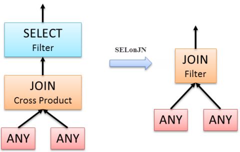
One example of a simple exploration rule is SELonJN, a rule that merges a suitable relational SELECT (row filter) into a logical join operation:

Another common exploration rule that generates a new logical alternative is JoinCommute:

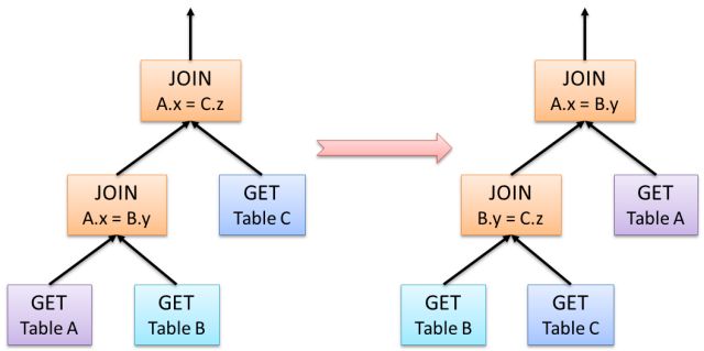
As the name suggests, JoinCommute explores a different logical join order, exploiting the fact that A JOIN B is equivalent to B JOIN A for inner joins.

Though logically equivalent, the different join orders may have different performance characteristics, once the logical alternatives are translated to a physical implementation by a later implementation rule.

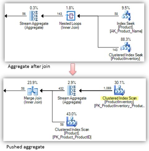
A third exploration rule that is relevant to our test query is GbAggBeforeJoin, a rule that explores the possibility of pushing an aggregation operation under a join:

Implementation Rule Examples

As mentioned, implementation rules transform part of a logical tree into a physical alternative:

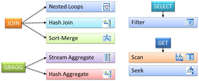
The diagram shows three join implementation rules, JNtoNL (nested loops), JNtoHS (hash join), JNtoSM (sort-merge); two implementations for Group-By Aggregate, GbAggToStrm (Stream Aggregate) and GbAggToHS (Hash Aggregate); along with SelectToFilter, GetToScan, and GetIdxToRng.

Which Rules Were Used?

If we want to see which rules were used when optimizing a query, one option is to use an undocumented view which shows the number of times a rule has been asked to estimate how valuable it might be in the current context (its ‘promise’ value), the number of times the rule was used to generate an alternative section of the tree (‘built’), and the number of times the output of the rule was successfully incorporated into the search space (‘succeeded’). A sample of the contents of this sys.dm_exec_query_transformation_stats DMV is shown below:

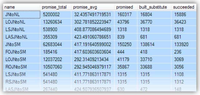
By taking a snapshot view of this information before and after optimizing a particular query, we can see which rules were run. The DMV is instance-wide however, so you would need to run these tests on a system to which you have exclusive access. The scripts that accompany this series of posts contain a complete test rig to show the rules used by each query.

End of Part 2

Part three in this series covers the Memo structure and optimization phases in detail.

Links to other parts of this series: Part 1 Part 3 Part 4